Lesson 2: Schedule Metrics & Diagnostics
Qualitative schedule reviews tell us what to look for — schedule performance metrics give us numbers to track. The four metrics covered in this lesson (CPLI, BEI, CEI, TFCI) are used in major infrastructure programmes to monitor schedule health, identify early warning signals, and support forensic analysis. They complement one another and should be read together rather than in isolation.
Prerequisite: These metrics rely on a properly structured, up-to-date CPM schedule. Poorly maintained schedules produce misleading metric values — always verify the underlying schedule quality first.
1. Critical Path Length Index (CPLI)
The Critical Path Length Index measures schedule efficiency — the relationship between the current critical path length and the time available to complete the project. It accounts for both the work remaining and the total float on the completion milestone.
Formula
CPLI = (CP Length + TF on Completion Milestone) ÷ CP Length
Target: ≥ 1.0
Interpreting the result:
Positive float on completion milestone — project is ahead of schedule. Low risk of delay.
Zero float on the completion milestone — project is exactly on schedule. No buffer remaining.
Negative float on completion milestone — the schedule predicts delayed completion. Immediate recovery planning required.

A CPLI trend chart plotted across data periods provides an early warning of project issues. A consistently declining CPLI — even if still above 1.0 — signals an erosion of schedule buffer that warrants early intervention.
2. Baseline Execution Index (BEI)
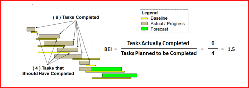
The Baseline Execution Index measures how well the project team is completing activities relative to the baseline plan. It compares actual completions to what was planned to be completed at the data date.
Formula
BEI = Tasks Actually Completed ÷ Tasks Planned to be Completed
Target: ≥ 1.0 (completing more than planned)

3. Current Execution Index (CEI)
The Current Execution Index is a snapshot-based metric. Rather than measuring against the baseline (as BEI does), CEI measures the proportion of activities that were forecast to finish within a given window that actually finished.
Formula
CEI = Tasks that Finished ÷ Tasks Forecasted to Finish
Maximum 1.0 | Target: > 0.80
Key characteristics of CEI:
- Maximum value of 1.0 — the denominator is set at the start of the window; activities finishing early in a later window do not increase CEI above 1.0 within the current window
- Target > 0.80 — a CEI below 0.80 signals significant execution slippage within the period
- Snapshot methodology — assessed at each reporting period by comparing forecast vs. actual finishes within that window only
At the data date, 37 activities were forecasted to finish in the reporting window. Of those, 29 actually finished.
CEI = 29 ÷ 37 = 0.78
Result: 0.78 — below the 0.80 target. This indicates the project team completed fewer activities than forecast during the period, warranting investigation into the causes of slippage.
4. Total Float Consumption Index (TFCI)
The Total Float Consumption Index measures how efficiently the project is consuming total float relative to the amount of work being performed. It compares actual duration consumed to the float consumed, indicating whether float is being "spent" appropriately.
Formula
TFCI = (AD + CPTF) ÷ AD
AD = Actual Duration | CPTF = Current Path Total Float | Target: ≥ 1.0
Actual Duration — calendar days elapsed from project start to data date
Current Path Total Float — total float on the critical path at the data date (negative if behind schedule)
≥ 1.0 (float not consumed faster than work progresses)
Worked example: At the data date, the project has been running for 763 calendar days. The critical path has −23 days of total float (i.e. the project is 23 days behind schedule).
A TFCI of 0.97 indicates the project is consuming float slightly faster than it is completing work — running 3% behind its efficiency target. While not yet critical, this trend warrants monitoring.


- Early project stage — TFCI has limited meaning early in the project when few activities have been completed and float patterns have not yet stabilised
- Delinquent projects only — most meaningful when the project is behind schedule (negative float). A project with positive float produces a TFCI > 1.0 regardless of actual performance quality
- Double-dipping risk — if as-built data is used to backfill activities, artificially inflated completions can produce misleading TFCI values
5. Program Rate Chart & Bow Wave Analysis
A Program Rate Chart displays the relationship between three completion lines and an Incomplete Tasks bar chart over the project timeline:
- Actual Finish — when activities actually completed (as-built)
- Baseline Finish — when activities were planned to complete (baseline)
- Forecast Finish — current schedule's predicted completion date for remaining activities
- Incomplete Tasks bars — the count of activities that remain incomplete at each reporting period

Bow Wave Analysis is a technique derived from Program Rate Charts. When the Forecast Finish line curves upward relative to the Baseline Finish line — resembling the bow wave of a ship — it indicates that planned activities are being pushed forward in time as successive data periods pass. The "bow wave" grows as work continues to slip from one period to the next without being completed.
6. Schedule Diagnostics
Schedule diagnostics go deeper than the DCMA 14-Point Assessment, examining the quality of schedule data across seven key categories. Diagnostics are typically performed using tools such as Microsoft Excel, Power BI, or Primavera P6 reporting functions to extract and interrogate schedule data.
Total number of activities versus project size — too few indicates inadequate detail; too many creates maintenance burden. Compare activity counts across reporting periods to detect unexplained additions or deletions.
Review activity durations for outliers — excessively long activities, activities with zero duration that are not milestones, and activities whose remaining durations have not changed between updates.
Activities with total float significantly exceeding their own duration are often indicators of missing logic. Compare duration and float values to identify activities that are effectively floating free of the network.
Identify and document all hard and soft constraints. Hard constraints (Must Start On, Must Finish On) override the CPM calculation and can produce misleading float values. Each constraint must be justified by a legitimate contract or site requirement.
Examine relationship types (FS, SS, FF, SF) across the schedule. An over-reliance on non-FS relationships can distort the critical path. Identify any SS or FF relationships being used as substitutes for proper activity logic.
Review all lags. Excessive or unexplained lags — particularly on SS or FF relationships — may conceal missing activities or inflate float. Each lag should be documented and independently justifiable.
Logic density = (number of relationships) ÷ (number of activities). Very low density (close to 1.0) suggests missing relationships. Very high density may indicate redundant or illogical ties. Well-structured schedules typically have a logic density between 1.2 and 2.0.
(CP Length + TF) ÷ CP Length — schedule efficiency. Target ≥ 1.0
Tasks Completed ÷ Tasks Planned — baseline adherence. Target ≥ 1.0
Tasks Finished ÷ Tasks Forecast to Finish — period execution. Target > 0.80, Max 1.0
(AD + CPTF) ÷ AD — float consumption efficiency. Target ≥ 1.0